Tutorial
To follow along with this tutorial in an interactive Python session, if you wish to do so, make sure you have downloaded the demonstration model “capacitor.mph” from this library’s GitHub repository, and saved it in the same folder from which you run Python.
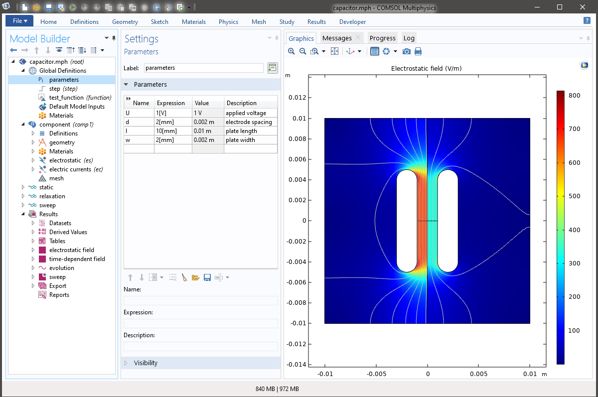
It is a model of a non-ideal, inhomogeneous, parallel-plate capacitor, in that its electrodes are of finite extent, the edges are rounded to avoid excessive electric-field strengths, and two media of different dielectric permittivity fill the separate halves of the electrode gap. Running the model only requires a license for the core Comsol platform, but not for any add-on module beyond that.
Starting Comsol
In the beginning was the client. And the client was with Comsol. And the client was Comsol. So let there be a Comsol client.
>>> import mph
>>> client = mph.Client(cores=1)
It takes roughly ten seconds until the client is initialized. In this example, the Comsol back-end is instructed to use only one processor core. If the optional parameter is omitted, it will use all cores available on the machine. Restricting this resource is useful when running several simulations in parallel. Note, however, that due to limitations of this library’s underlying Python-to-Java bridge, you cannot instantiate the Client class more than once. If you wish to accomplish that, in order to realize the full compute power of your simulation hardware, you need to start separate Python sessions, one for each client.
Managing models
Now that we have the client up and running, we can tell it to load a model file.
>>> model = client.load('capacitor.mph')
It returns a model object, i.e. an instance of the
Model class. We will learn what to do with it
further down. For now, it was simply loaded into memory. We can
list the names of all models the client currently manages.
>>> client.names()
['capacitor']
If we were to load more models, that list would be longer. Note that the above simply displays the names of the models. The actual model objects can be recalled as follows:
>>> client.models()
[<mph.model.Model object at 0x000002CAF6C0BE80>]
We will generally not need to bother with these lists, as we would
rather hold on to the model reference we received from the client.
But to free up memory, we could remove a specific model.
>>> client.remove(model)
Or we could remove all models at once — restart from a clean slate.
>>> client.clear()
>>> client.names()
[]
Inspecting models
Let’s have a look at the parameters defined in the model.
>>> for parameter in model.parameters():
...     print(parameter)
...
parameter(name='U', value='1[V]', description='applied voltage')
parameter(name='d', value='2[mm]', description='electrode spacing')
parameter(name='l', value='10[mm]', description='plate length')
parameter(name='w', value='2[mm]', description='plate width')
Or the materials for that matter.
>>> model.materials()
['medium 1', 'medium 2']
They will be used by these physics interfaces:
>>> model.physics()
['electrostatic', 'electric currents']
To solve the model, we will run these studies:
>>> model.studies()
['static', 'relaxation', 'sweep']
Notice something? All features are referred to by their names, also
known as labels, such as medium 1. But not by their tags, such as
mat1, which litter not just the Comsol programming interface, but,
depending on display settings, its graphical user interface as well.
Tags are an implementation detail. An unnecessary annoyance to anyone who has ever scripted a Comsol model from either Matlab or Java. Unnecessary because names/labels are equally enforced to be unique, so tags are not needed for disambiguation. And annoying because we cannot freely change a tag. Say, we remove a feature, but then realize we need it after all, and thus recreate it. It may now have a different tag. And any code that references it has to adapted.
This is Python though. We hide implementation details as much as we can. Abstract them out. So refer to things in the model tree by what you name them in the model tree. If you remove a feature and then put it back in, just give it the same name, and nothing has changed. You may also set up different models to be automated by the same script. No problem, as long as your naming scheme is consistent throughout.
Modifying parameters
As we have learned from the list above, the model defines a parameter
named d that denotes the electrode spacing. If we know a parameter’s
name, we can access its value directly.
>>> model.parameter('d')
'2[mm]'
If we pass in not just the name, but also a value, that same method modifies it.
>>> model.parameter('d', '1[mm]')
>>> model.parameter('d')
'1[mm]'
This particular model’s only geometry sequence
>>> model.geometries()
['geometry']
is set up to depend on that very value. So it will effectively change the next time it is rebuilt. This will happen automatically once we solve the model. But we may also trigger the geometry rebuild right away.
>>> model.build()
Running simulations
To solve the model, we need to create a mesh. This would also be taken care of automatically, but let’s make sure this critical step passes without a hitch.
>>> model.mesh()
Now run the first study, the one set up to compute the electrostatic solution, i.e. the instantaneous and purely capacitive response to the applied voltage, before leakage currents have any time to set in.
>>> model.solve('static')
This modest simulation should not take longer than a few seconds. While we are at it, we may as well solve the remaining two studies, one time-dependent, the other a parameter sweep.
>>> model.solve('relaxation')
>>> model.solve('sweep')
They take a little longer, but not much. We could have solved all three studies at once, or rather, all of the studies defined in the model.
>>> model.solve()
Evaluating results
Let’s see what we found out and evaluate the electrostatic capacitance, i.e. at zero time or infinite frequency.
>>> model.evaluate('2*es.intWe/U^2', 'pF')
array(1.31947349)
All results are returned as NumPy arrays. Though scalars such as this
one could be readily cast to a (regular Python) float.
We could also ask where the electric field is strongest.
>>> (x, y, E) = model.evaluate(['x', 'y', 'es.normE'])
>>> E.max()
1455.5010798501924
>>> imax = E.argmax()
>>> x[imax], y[imax]
(-0.0005161744830262844, 0.004178390490229011)
Note how this time we did not specify any units. When left out, values are returned in default units. Here specifically, the maximum field strength in V/m and its coordinates in meters.
We also did not specify the dataset, even though there are three different studies that have separate solutions and datasets associated along with them. When not named specifically, the default dataset is used. That generally refers to the study defined first, here “static”. The default dataset is the one resulting from that study, here — inconsistently — named “electrostatic”.
>>> model.datasets()
['electrostatic', 'time-dependent', 'parametric sweep']
Now let’s look at the time dependence. The two media in this model have a small, but finite conductivity, leading to leakage currents in the long run. As the two conductivities also differ in value, charges will accumulate at the interface between the media. This interface charge leads to a gradual relaxation of the total capacitance over time. We can tell that from its value at the first and last time step.
>>> C = '2*ec.intWe/U^2'
>>> model.evaluate(C, 'pF', 'time-dependent', 'first')
array(1.31947349)
>>> model.evaluate(C, 'pF', 'time-dependent', 'last')
array(1.48410629)
The “first” and “last” time step defined in that study are 0 and 1 second, respectively.
>>> (indices, values) = model.inner('time-dependent')
>>> values[0]
0.0
>>> values[-1]
1.0
Obviously, the capacitance also varies if we change the distance between the electrodes. In the model, a parameter sweep was used to study that. These “outer” solutions, just like the time-dependent “inner” solutions, are referenced by indices, i.e. integer numbers, each of which corresponds to a particular parameter value.
>>> (indices, values) = model.outer('parametric sweep')
>>> indices
array([1, 2, 3], dtype=int32)
>>> values
array([1., 2., 3.]
>>> model.evaluate(C, 'pF', 'parametric sweep', 'first', 1)
array(1.31947349)
>>> model.evaluate(C, 'pF', 'parametric sweep', 'first', 2)
array(0.73678503)
>>> model.evaluate(C, 'pF', 'parametric sweep', 'first', 3)
array(0.52865545)
Then again, with a scripting interface such as this one, we may as well run the time-dependent study a number of times and change the parameter value from one run to the next. General parameter sweeps can get quite complicated in terms of how they map to indices as soon as combinations of parameters are allowed. Support for this may therefore be dropped in a future release — while the API is still considered unstable, which it is for as long as the version number of this library does not start with a 1 —, just to keep things simple and clean.
Saving results
To save the model we just solved, along with its solution, just do:
>>> model.save()
This would overwrite the existing file we loaded the model from. To avoid this, we could specify a different file name.
>>> model.save('capacitor_solved')
The .mph extension will be added automatically if it is not included
in the first place.
Maybe we don’t actually need to keep the solution and mesh data around. The model was quick enough to solve, and we do like free disk space. We would just like to be able to look up modeling details somewhere down the line. Comsol also keeps track of the modeling history: a log of which features were created, deleted, modified, and in which order. Typically, such details are irrelevant. We can prune them by resetting that record.
>>> model.clear()
>>> model.reset()
>>> model.save('capacitor_compacted')
Most functionality that the library offers is covered in this tutorial. The few things that were left out can be gleaned from the API documentation.